Walkthrough particle diffusing in water

In this walkthrough we will explore the potential of WISE for the analysis of micron-sized particles diffusing in water. We will use images from https://soft-matter.github.io/trackpy/tutorial/walkthrough.html, detect and track the particles, and compare our result to the one obtained by the trackpy team.

Setup

import os
import datetime
import numpy as np

import astropy.units as u

import wise
from wise import tasks
from libwise import imgutils, plotutils, nputils, presetutils

%matplotlib gtk

ctx = wise.AnalysisContext()

Setting up the data configuration:

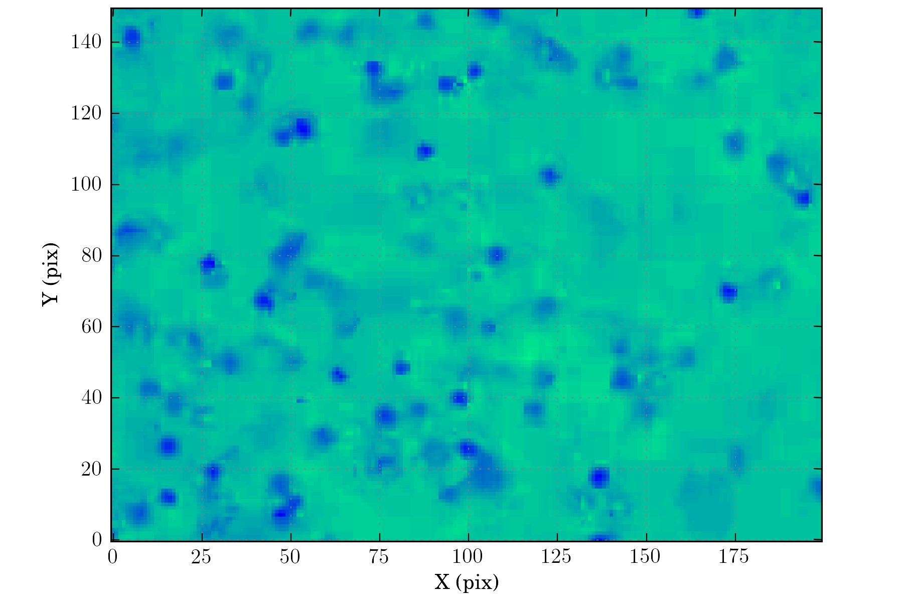
The full data set is composed of 300 images. We will first analyse only part of it. We use a k sigma estimator to estimate the noise level in the images:

BASE_DIR = os.path.expanduser("~/data/bulk_water")

def get_bg(self, img):
    return nputils.k_sigma_noise_estimation(img.data)

def pre_process(self, img):
    img.resize((150, 200))
    img.data = 255 - img.data

ctx.config.data.data_dir = os.path.join(BASE_DIR, "run001")
ctx.config.data.bg_fct = get_bg
ctx.config.data.pre_process_fct = pre_process
ctx.config.data.projection_relative = False

ctx.select_files(os.path.join(BASE_DIR, 'data/*0[0-9][0-9].png'), step=5)

Number of files selected: 20

tasks.view_all(ctx, cmap=plotutils.get_cmap('winter_r'))

Setting up the detection configuration:

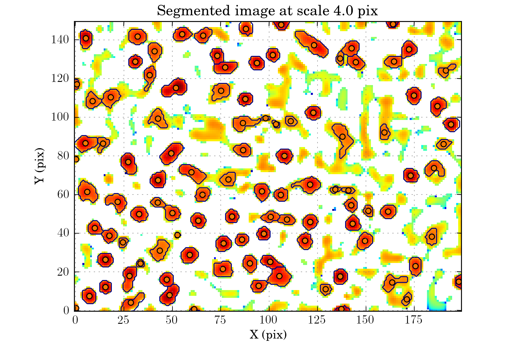
We want to track only the most prominent particles, and to control it we set an high value for alpha_detection. Also the particles are typically all of the same sizes, and the displacement from image to image is small, so we can perform the analysis only on one scale of the wavelet decomposition:

ctx.config.finder.min_scale = 2
ctx.config.finder.max_scale = 3
ctx.config.finder.exclude_noise = False
ctx.config.finder.alpha_detection = 15
ctx.config.finder.alpha_threashold = 10
ctx.config.finder.ms_dec_klass = wise.WaveletMultiscaleDecomposition

tasks.detection_all(ctx)

tasks.view_wds(ctx, num=False)

Setting up the matching configuration:

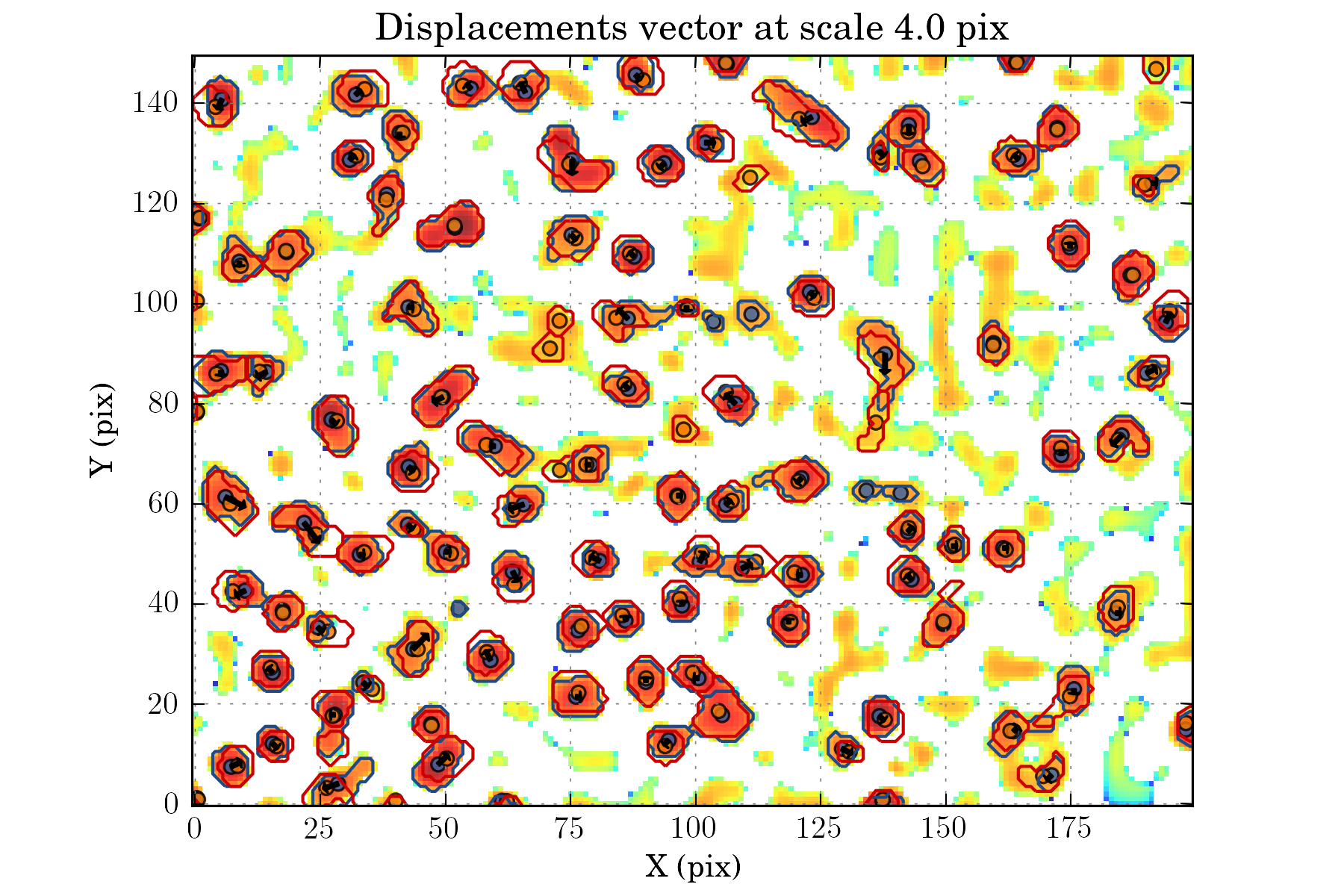
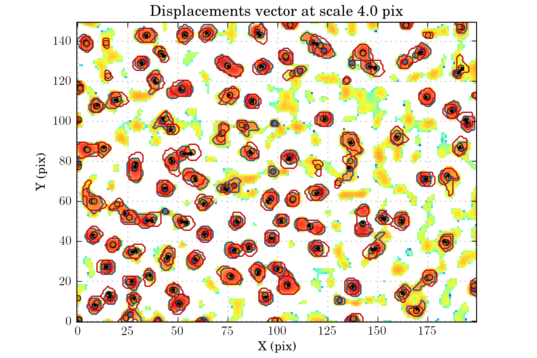
A reasonable maximum displacement from image to image is 5 pixels. For this tests, we do not needs the extra features of ScaleMatcherMSCSC2, and we can use the more simple and faster ScaleMatcherMSCI matcher:

ctx.config.matcher.maximum_delta = 5
ctx.config.matcher.mscsc2_smooth = False
ctx.config.matcher.ignore_features_at_border = True
ctx.config.matcher.method_klass = wise.ScaleMatcherMSCI

tasks.match_all(ctx)

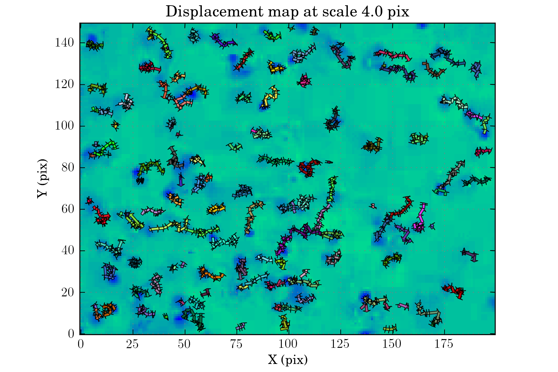
tasks.view_displacements(ctx, 4)

tasks.view_links(ctx, map_cmap='winter_r')

Assessing the results:

To assess the performance of WISE, we will now compare our results to the one obtain by trackpy. We will first re run the matching with a more complete data set:

def pre_process(self, img):
    img.data = 255 - img.data

ctx.config.data.pre_process_fct = pre_process

ctx.select_files(os.path.join(BASE_DIR, 'data/*.png'), step=5)

Number of files selected: 60

tasks.match_all(ctx)

The different plotting tasks of WISE all have an option to save the plot in a file. We will use it to view the trajectories of all the particles:

presetutils.set_rc_preset('presentation', {'figure.figsize': (10, 7)})
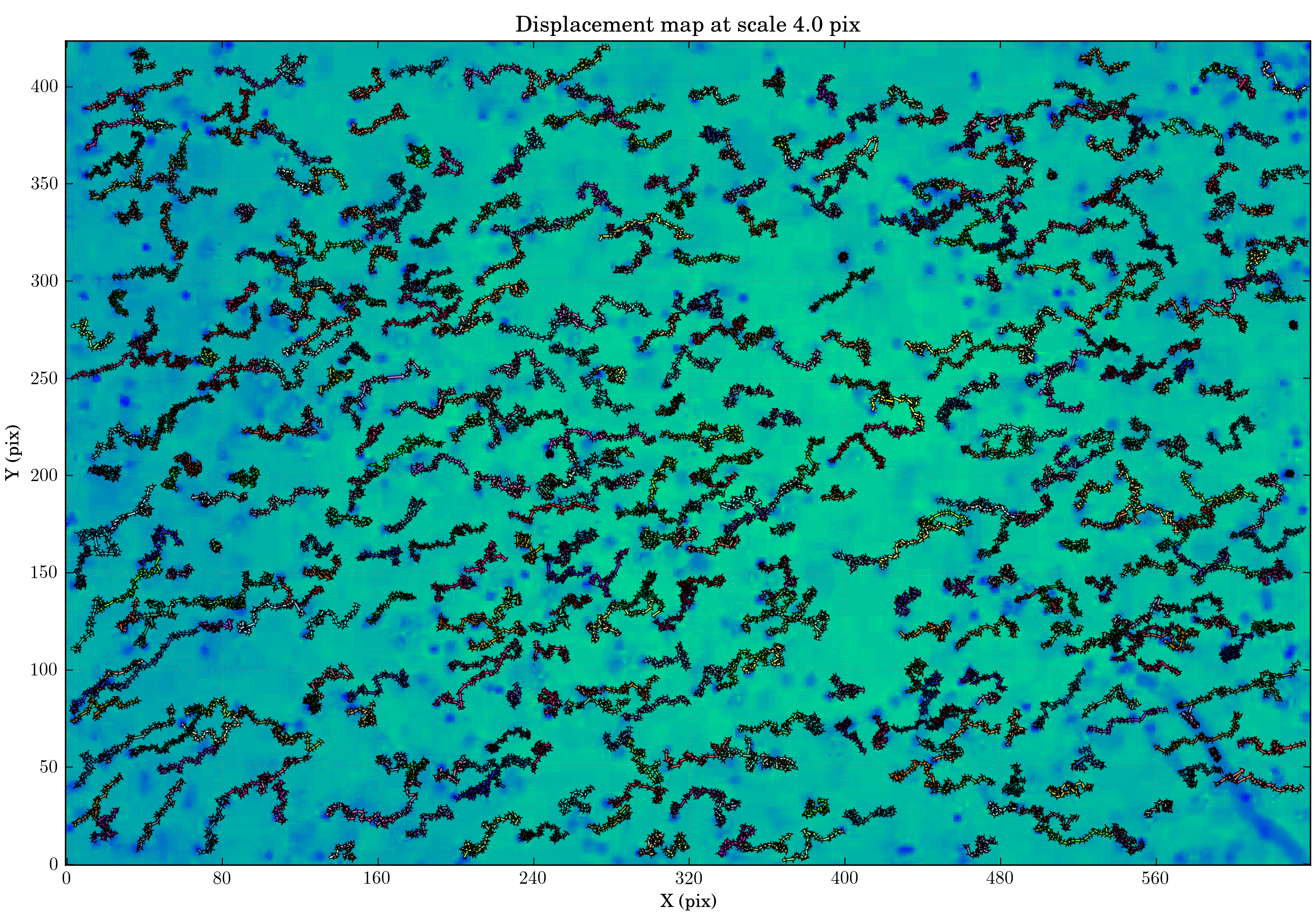
tasks.view_links(ctx, save_filename='view_links_full.png', min_link_size=40, map_cmap='winter_r')
presetutils.set_rc_preset('display')

Now to compare our result, we will use analysis method developed by trackpy to obtain the mean square displacement of the particles. The following will convert WISE result data structure into one compatible with trackpy:

import trackpy as tp
import pandas as pd
from uncertainties import ufloat

data = tasks.get_velocities_data(ctx, min_link_size=40)

get_link_id = np.vectorize(lambda link_id: np.int(link_id[2:]))
frame = data['epoch'].values
x = data['ra'].values
y = data['dec'].values
link_id = get_link_id(data['link_id'].values)
data_tp = pd.DataFrame(np.array([x, y, frame, link_id]).T, columns=['x', 'y', 'frame', 'particle'])
data_tp = data_tp.drop_duplicates()

%matplotlib inline

To make sure that the conversion was correctly done, we first plot the particle trajectories:

tp.plot_traj(data_tp)

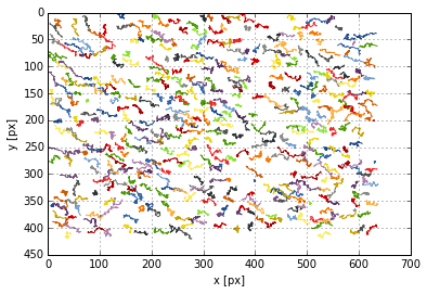
<matplotlib.axes._subplots.AxesSubplot at 0x7f96185c9290>

This will remove the overall drift:

d = tp.compute_drift(data_tp)
tm = tp.subtract_drift(data_tp, d)

This will compute the mean squared displacement of each particle and plot MSD vs. lag time:

im = tp.imsd(tm, 100/285., 24/5.)
ax = im.plot(loglog=True, style='k-', alpha=0.1, legend=False)
ax.set_ylabel(r'$\langle \Delta r^2 \rangle$ [$\mu$m$^2$]');

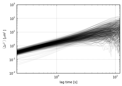
And now we can compute the ensemble mean squared displacement and compare it with the theoretical one:

#em = tp.emsd(tm, 100/285., 24/5.)
ax = em.plot(loglog=True, style='ro')

fit_fct = nputils.PowerFct1.fit(em.index, em.values)
plotutils.plot_fit(ax, em.index, em.values, fit_fct)

print "n = ", ufloat(fit_fct.a, fit_fct.ea)
print "A = ", ufloat(fit_fct.b, fit_fct.eb)

n =  1.0636+/-0.0024
A =  1.734+/-0.007

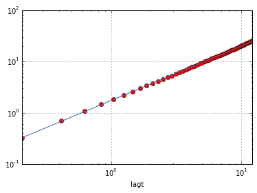
Theory of particles diffusivity in water predict A = 1.74 and n = 1.